Perlin Noise has been a mainstay of computer graphics since 1985 [EBERT98],[FOLEY96],[PERLIN85], being the core procedure that enables procedural shaders to produce natural appearing materials. Now that real-time graphics hardware has reached the point where memory bandwidth is more of a bottleneck than is raw processing power, it is imperative that the lessons learned from procedural shading be adapted properly to real-time hardware platforms.
The original implementation of Noise is fairly simple. First I will show how it is constructed, and various ways it is used in shader programs to get different kinds of procedural textures. There will be pictures and animations. Then I'll talk about several approaches to real-time implementation, so that Noise can be used most effectively in game hardware and other platforms that should support Noise-intensive imagery at many frames per second.
Noise is a mapping from Rn to R - you input an n-dimensional point with real coordinates, and it returns a real value. Currently the most common uses are for n=1, n=2, and n=3. The first is used for animation, the second for cheap texture hacks, and the third for less-cheap texture hacks. Noise over R4 is also very useful for time-varying solid textures, as I'll show later.
Noise is band-limited - almost all of its energy (when looked at as a signal) is concentrated in a small part of the frequency spectrum. High frequencies (visually small details) and low frequencies (large shapes) contribute very little energy. Its appearance is similar to what you'd get if you took a big block of random values and blurred it (ie: convolved with a gaussian kernel). Although that would be quite expensive to compute.
First I'll outline the ideal characteristics of a Noise function, then I'll review how the original Noise function matches these characteristics (sort of). After that I'll outline how one might implement the original Noise function in hardware, in an optimized way. Finally, I'll show a radically different approach I've been taking to implementing Noise, with an eye toward standardizing on a visually better primitive that can also run much faster in hardware.
There are two major issues involved in this adaptation: (i) A common procedural shading abstract machine language, to enable the capabilities that were first introduced in [Perlin85], and subsequently adapted by the motion picture special effects industry, and (ii) a standard, fast, robust, differentiable and extensible Noise function contained in the instruction set of this abstract machine language. This chapter addresses the second of these two issues.
The ideal Noise can be separated from the shortcomings of any particular implementation which aims to approximate this ideal. [Perlin85] outlined a number of characteristics for an ideal Noise. Ideally a hardware-implemented standard would conform to this ideal, without suffering from any shortcomings.
The traditional Noise algorithm, while very useful, had some shortcomings that would be of particular consequence in a real-time setting and in a hardware implementation. I'll describe a new method that suffers from none of these shortcomings. Shortcomings which are addressed include:
Specifically, when these implementations of Noise are applied to a rotated domain, a casual viewer of the result can easily pick out the orientation of the rotated coordinate grid. Ideally, it should be impossible for a casual viewer to infer the orientation of the rotated coordinate system, when presented with the texture image produced by Noise applied to a rotated domain.
In non-real time applications, in which perfection of the final result is far more important than is processing budget, such as is the case in the use of Noise for motion picture special effects, it is possible to "fudge" some these artifacts by applying Noise multiple times. For example, as I mentioned in my previous chapter, the procedural shaders for the scene depicting ocean waves in the recent film "The Perfect Storm" combined about 200 shader procedures, each of which invoked Perlin Noise. In contrast, for real-time applications, where the cost of every evaluation counts, it is crucial that Noise itself be artifact free, that its derivative be directly computable, and that it incur a relatively small computational cost.

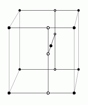
In three dimensions, there are eight surrounding grid points. To combine their respective influences we use a trilinear interpolation (linear interpolation in each of three dimensions).
In practice this means that once we've computed the 3t2-2t3 cross-fade function in each of x,y and z, respectively, then we'll need to do seven linear interpolations to get the final result. Each linear interpolation a+t(b-a) requires one multiply.
In the diagram, the six white dots are the results of the first six interpolations: four in x, followed by two in y. Finally, one interpolation in z gives the final result
To compute the pseudo-random gradient, we can first precompute a table of permutations P[n], and a table of gradients G[n]:
G = G[ ( i + P[ (j + P[k]) mod n ] ) mod n ]
A speedier variation would be to let n be a power of two. Then, except for bit masking (which is essentially free), the computation reduces to:
G = G[ i + P[ j + P[ k ] ] ]
For review, here is a very short set of representative examples to show how Noise can be used to make interesting textures.
| noise sin(x+sum 1/f( |noise| )) | |
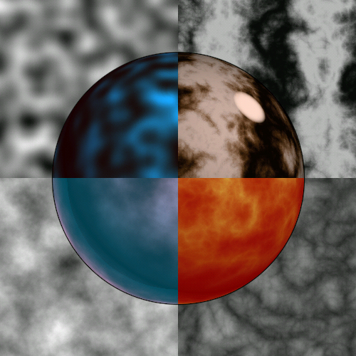
| sum 1/f(noise) | sum 1/f( |noise| ) |
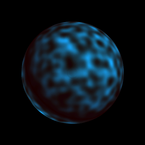
noise
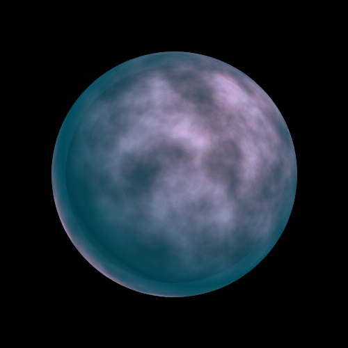
sum 1/f(noise)
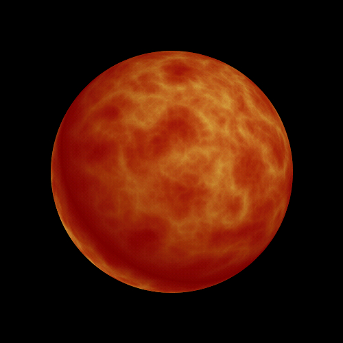
sum 1/f( |noise|)
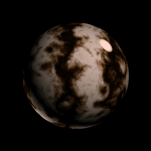
sin(x + sum 1/f( |noise| ))
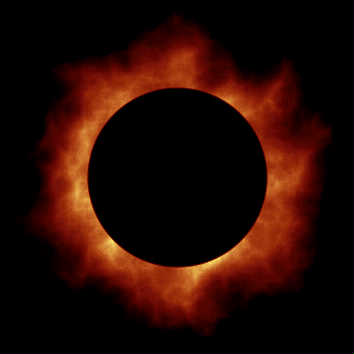
Flame: Noise scales in x,y, translates in z

Clouds: Noise translates in x and z
Creating these textures is really quite simple. Below is an image of the gradient field used to create the cloud texture, before perturbation:

Clouds without 1/f(|noise|) perturbation
But ideally one would like to implement Noise as a primitive operation, directly in hardware, so that it may be invoked as many times as possible, at the texture sample evaluation level, without becoming a computational bottleneck, and perhaps even for volume filling textures [PERLIN89]. What would this require?
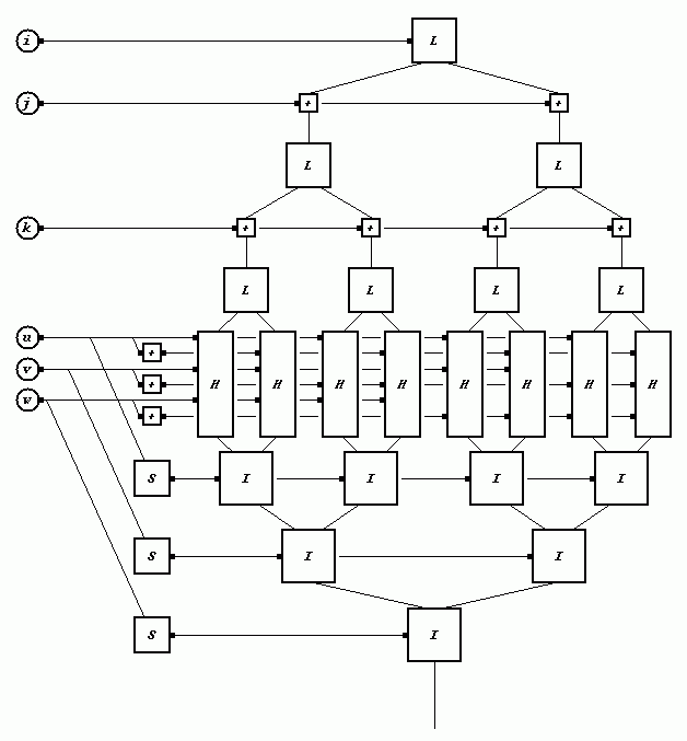
I found that it could be fairly inexpensive, if you worked with a restricted bit depth. For example, if you assume an 8.8 bit input in each of X,Y,Z (ie: each component is in a tiling integer lattice which is 256 units on a side, and there are 256 domain steps within each unit), and an 8 bit output range, then you can implement Noise in under 10K gates, which is a remarkably small number.
The basic approach is to do a pipelined architecture, as in the diagram below. In that diagram:
The module can be pipelined so that a new Noise evaluation can be calculated at each clock cycle, with a latency of about twenty clock cycles.
The image below is a side-by-side visual comparison of "traditional" Noise with the method described here. The four quadrants of the image represent, respectively:
| df/dx = d(Noise(xyz))/dx | df/dy = d(Noise(xyz))/dy |
|---|---|
| df/dz = d(Noise(xyz))/dz | f(xyz) = Noise(xyz) |
Each of these quadrants is divided into four sub-quadrants. These represent, respectively:
| old Noise at z = 0 | new Noise at z = 0 |
|---|---|
| old Noise at z = 0.5 | new Noise at z = 0.5 |
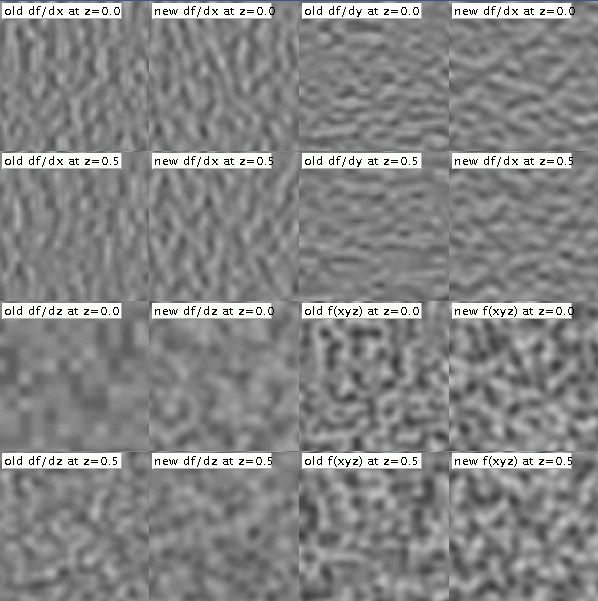
The old and new Noise look roughly the same when evaluated at z=0, the major visual difference being that the new Noise implementation is visually isotropic. Specifically, if the picture is arbitrarily rotated, it is not possible for an observer examining any subportion of the resulting texture to infer, by visual examination, the original orientation of the image produced by new Noise, whereas it is possible for an observer to infer this orientation for the image produced by the old Noise.
Note also the appearance of the derivative with respect to z. In the old Noise this degenerates into an image of fuzzy squares.
Below is the same comparison, this time with the domain magnified by a factor of four. Note the artifacts in df/dx and in df/dy in old Noise, which appear as thin vertical streaks in df/dx and as thin horizontal streaks in df/dy. This is due to the use of the piecewise cubic interpolant function 3 t2 - 2 t3, whose derivative is 6 t - 6 t2, which contains a linear term. The presence of this linear term causes the derivative of the Noise function to be discontinuous at cubic cell boundaries.
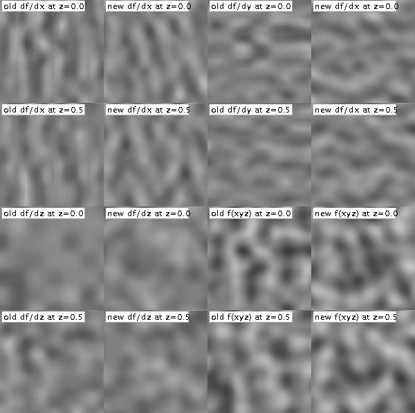
Rather than using a tricubic interpolation function, this interpolation scheme uses a spherically symmetric kernel, multiplied by a linear gradient, at each component surrounding vertex. This confers three advantages:
Rather than using inner products, with their attendent (and expensive) multiplies, to convert each index into an actual pseudo-random gradient, the new reconstruction method uses a method that produces more visually uniform results, and is easier to integrate into a derivative calculation, while requiring no multiplies at all.
Each of these changes is now described in more detail:
Given an integer lattice point (i,j,k), the new method uses a bit-manipulation algorithm to generate a six bit quantity. This six bit quantity is then used to generate a gradient direction. The six bit quantity is defined as the lower six bits of the sum:
   b(i,j,k,0) + b(j,k,i,1) + b(k,i,j,2) + b(i,j,k,3) +
   b(j,k,i,4) + b(k,i,j,5) + b(i,j,k,6) + b(j,k,i,7)
where b() uses its last argument as a bit index into a very small table of bitPatterns.
   define b(i,j,k,B) :
      patternIndex = 4 * bitB(i) + 2 * bitB(j) + bitB(k)
      return bitPatterns[patternIndex]
and where the bit pattern table is defined as:
bitPatterns[] = { 0x15,0x38,0x32,0x2c,0x0d,0x13,0x07,0x2a }
Using index to derive pseudorandom gradient
The new method converts a six bit pseudo-random index into a visually uniform gradient vector which is easy to integrate into a derivative calculation and which requires no multiplies to compute. The key innovation is to use values of only zero or one for the gradient magnitude.
The specific new technique is as follows: The six bit index is split into (i) a lower three bit quantity, which is used to compute a magnitude of either zero or one for each of x,y and z, and (ii) an upper three bit quantity, which is used to determine an octant for the resulting gradient (positive or negative sign in each of x,y, and z).
(i) Magnitude computation, based on the three lower bits:
If bit1bit0 = 0, then let (p,q,r) = (x,y,z). Otherwise, let (p,q,r) be a rotation of the order of (x,y,z) to (y,z,x) or (z,x,y), as bit1bit0 = 1 or 2, respectively, and set either q or r to zero as bit2 = 0 or 1, respectively. The resulting possible rotations are shown in the table below:
| bit2bit1bit0 | bit2bit1bit0 | ||||||||||||||
|---|---|---|---|---|---|---|---|---|---|---|---|---|---|---|---|
| 000 | p=x q=y r=z | 100 | p=x q=y r=z
| 001 | p=y q=z r=0
| 101 | p=y q=0 r=x
| 010 | p=z q=x r=0
| 110 | p=z q=0 r=y
| 011 | p=x q=y r=0
| 111 | p=x q=0 r=z
| |
(ii) Octant computation, based on the three upper bits:
Once p,q,r have been determined, invert the sign of p if bit5=bit3, of q if bit5=bit4, and of r if bit5=(bit4!=bit3), then add together p,q, and r. The resulting possible gradient values are shown in the table below:
| bit5bit4bit3 | bit5bit4bit3 | ||||||||||||||
|---|---|---|---|---|---|---|---|---|---|---|---|---|---|---|---|
| 000 | -p-q+r | 100 | p+q-r
| 001 | p-q-r
| 101 | -p+q+r
| 010 | -p+q-r
| 110 | p-q+r
| 011 | p+q+r
| 111 | -p-q-r
| |
In this way, a gradient vector is defined using only a small number of bit operations and two additions. In particular, the computation of gradient requires no multiply operations. This contrasts very favourably with previous implementations of Noise, in which three multiply operations were required for each gradient computation (one multiply in each of the three component dimensions).
Rather than placing each input point into a cubic grid, based on the integer parts of its (x,y,z) coordinate values, the input point is placed onto a simplicial grid as follows:
   define skew((x,y,z) -> (x',y',z')) :
      s = (x+y+z)/3
      (x',y',z') = (x+s,y+s,z+s)
This
skew transformation linearly scales about the origin, along the x=y=z axis,
bringing the point (1,1,1) to the point (2,2,2).
(i',j',k') = ( floor(x'),floor(y'),floor(z') )
This corner point can be converted back to the original unskewed coordinate system via:
   define unskew((i',j',k') -> (i,j,k)) :
      s' = (i'+j'+k')/6
      (i,j,k) = (i-s',j-s',k-s')
Also consider the original coordinates relative to the
unskewed image of the cube corner:
(u,v,w) = ( x-i, y-j, z-k )
   { (0,0,0) , (1,0,0) , (1,1,0) , (1,1,1) }
   { (0,0,0) , (1,0,0) , (1,0,1) , (1,1,1) }
   { (0,0,0) , (0,1,0) , (1,1,0) , (1,1,1) }
   { (0,0,0) , (0,1,0) , (0,1,1) , (1,1,1) }
   ( (0,0,0) , (0,0,1) , (1,0,1) , (1,1,1) }
   { (0,0,0) , (0,0,1) , (0,1,1) , (1,1,1) }
Each of these simplices can be defined as an ordered
traversal A,B,C from vertex (0,0,0) to vertex (1,1,1) of a unit cube
in the skewed space, where { A,B,C } is some permutation of
{ (1,0,0),(0,1,0),(0,0,1) }.
For example, the last simplex above can be defined as an z,y,x traversal,
since its first transition A = (0,0,1),
its second transition B = (0,1,0), and
its third transition C = (0,0,1).
Which simplex contains the input point is determined by the relative magnitudes of u, v and w. For example, if w > v and v > u, then the first transition will be in the z dimension, so A = (0,0,1), and the second transition will be in the y dimension, so B = (0,1,0). In this case, the point lies within the simplex whose traversal order is z,y,x.
The four surrounding vertices of the simplex can now be defined as:
{ (i,j,k), (i,j,k)+unskew(A), (i,j,k)+unskew(A+B), (i,j,k)+unskew(A+B+C) }
Spherical kernel
If the input point is positioned (u,v,w) from a given simplex vertex, then the contribution from that vertex to the final result will be given by:
   t = 0.6 - (u2 + v2 + w2)
   if t > 0 then 8(t4) else 0
Any implementation needs to choose the number of bits of accuracy desired for both input and for output. This choice of bit-depth will vary the number of hardware gates required, but does not in any significant way modify the underlying technique.
In a pipelined implementation, it is very straightforward to maintain a high performance relative to the number of hardware gates used in the implementation, by pipelining the input. This guarantees that the circuitry which implements each different part of the method is always in active use.
The hardware circuitry that implements the new method can make use of an efficiently pipelined parallel implementation, as follows:
It is straightforward to generalize this approach to higher dimensions. In n dimensions, a hypercube can be decomposed into n! simplices, where each simplex corresponds to an ordering of the edge traversal of the hypercube from its lower vertex (0,0,...0) to its upper vertex (1,1,...1). For example, when n=4, there are 24 such traversal orderings. To determine which simplex surrounds the input point, one must sort the coordinates in the difference vector (u1,...un) from the lower vertex of the surrounding skewed hypercube to the input point.
For a given n, the "skew factor" f should be set to f = (n+1)½, so that the point (1,1,...1) is transformed to the point (f,f,...f). In addition, the exact radius and amplitude of the hypersphere-shaped kernel centered at each simplex vertex need to be tuned so as to produce the best visual results for each choice of n.
Previous implementations of Noise, since they were defined on a cubic grid, required a successive doubling of the number of grid points that need to be visited, for each increment in the number of dimensions n. The computational complexity, in terms of vector operations, required to evaluate Noise in n dimensions was therefore O(2n). Since this is exponential in the number of dimensions, it is not practical beyond a few dimensions.
In contrast, the new implementation , since it is defined on a simplicial grid, requires only an increment in the number of grid points that need be visited, for each increment in the number of dimensions n. The computationational complexity, in terms of vector operations, required to evaluate the new implementation of Noise in n dimensions is therefore O(n). Since this is only polynomial in the number of dimensions, it is practical even for higher dimensions.
To compute the computational complexity in terms of arithmetic operations, both of the above figures need to be multiplied by O(n), since the length of each contributing vector operation, and therefore the computational cost of each vector operation, is n, increasing linearly with the number of dimensions. Therefore the computational complexity of previous Noise implementations in n dimensions is O(n 2n), whereas the computational complexity of the new Noise implementation, in n dimensions is O(n2).
The important conclusion to be drawn from this analysis is that this new implementation of Noise, in contrast to previous implementations, is practical in even high dimensional spaces, because it is a computation of only polynomial complexity, not of exponential complexity. For example, the cost of computing Noise in 10 dimensions using previous implementations is approximately O(10 * 210) = O(10240), whereas the cost using the new implementation is approximately O(10 * 10) = O(100). In this case, a computational advantage factor of 100 is demonstrated. A reference Java implementation of the new Noise algorithm is given below, in Appendix B.
/* coherent noise function over 1, 2 or 3 dimensions */
/* (copyright Ken Perlin) */

#include <stdlib.h>
#include <stdio.h>
#include <math.h>

#define B 0x100
#define BM 0xff

#define N 0x1000
#define NP 12   /* 2^N */
#define NM 0xfff

static p[B + B + 2];
static float g3[B + B + 2][3];
static float g2[B + B + 2][2];
static float g1[B + B + 2];
static start = 1;

static void init(void);

#define s_curve(t) ( t * t * (3. - 2. * t) )

#define lerp(t, a, b) ( a + t * (b - a) )

#define setup(i,b0,b1,r0,r1)\
	t = vec[i] + N;\
	b0 = ((int)t) & BM;\
	b1 = (b0+1) & BM;\
	r0 = t - (int)t;\
	r1 = r0 - 1.;

double noise1(double arg)
{
	int bx0, bx1;
	float rx0, rx1, sx, t, u, v, vec[1];

	vec[0] = arg;
	if (start) {
		start = 0;
		init();
	}

	setup(0, bx0,bx1, rx0,rx1);

	sx = s_curve(rx0);

	u = rx0 * g1[ p[ bx0 ] ];
	v = rx1 * g1[ p[ bx1 ] ];

	return lerp(sx, u, v);
}

float noise2(float vec[2])
{
	int bx0, bx1, by0, by1, b00, b10, b01, b11;
	float rx0, rx1, ry0, ry1, *q, sx, sy, a, b, t, u, v;
	register i, j;

	if (start) {
		start = 0;
		init();
	}

	setup(0, bx0,bx1, rx0,rx1);
	setup(1, by0,by1, ry0,ry1);

	i = p[ bx0 ];
	j = p[ bx1 ];

	b00 = p[ i + by0 ];
	b10 = p[ j + by0 ];
	b01 = p[ i + by1 ];
	b11 = p[ j + by1 ];

	sx = s_curve(rx0);
	sy = s_curve(ry0);

#define at2(rx,ry) ( rx * q[0] + ry * q[1] )

	q = g2[ b00 ] ; u = at2(rx0,ry0);
	q = g2[ b10 ] ; v = at2(rx1,ry0);
	a = lerp(sx, u, v);

	q = g2[ b01 ] ; u = at2(rx0,ry1);
	q = g2[ b11 ] ; v = at2(rx1,ry1);
	b = lerp(sx, u, v);

	return lerp(sy, a, b);
}

float noise3(float vec[3])
{
	int bx0, bx1, by0, by1, bz0, bz1, b00, b10, b01, b11;
	float rx0, rx1, ry0, ry1, rz0, rz1, *q, sy, sz, a, b, c, d, t, u, v;
	register i, j;

	if (start) {
		start = 0;
		init();
	}

	setup(0, bx0,bx1, rx0,rx1);
	setup(1, by0,by1, ry0,ry1);
	setup(2, bz0,bz1, rz0,rz1);

	i = p[ bx0 ];
	j = p[ bx1 ];

	b00 = p[ i + by0 ];
	b10 = p[ j + by0 ];
	b01 = p[ i + by1 ];
	b11 = p[ j + by1 ];

	t  = s_curve(rx0);
	sy = s_curve(ry0);
	sz = s_curve(rz0);

#define at3(rx,ry,rz) ( rx * q[0] + ry * q[1] + rz * q[2] )

	q = g3[ b00 + bz0 ] ; u = at3(rx0,ry0,rz0);
	q = g3[ b10 + bz0 ] ; v = at3(rx1,ry0,rz0);
	a = lerp(t, u, v);

	q = g3[ b01 + bz0 ] ; u = at3(rx0,ry1,rz0);
	q = g3[ b11 + bz0 ] ; v = at3(rx1,ry1,rz0);
	b = lerp(t, u, v);

	c = lerp(sy, a, b);

	q = g3[ b00 + bz1 ] ; u = at3(rx0,ry0,rz1);
	q = g3[ b10 + bz1 ] ; v = at3(rx1,ry0,rz1);
	a = lerp(t, u, v);

	q = g3[ b01 + bz1 ] ; u = at3(rx0,ry1,rz1);
	q = g3[ b11 + bz1 ] ; v = at3(rx1,ry1,rz1);
	b = lerp(t, u, v);

	d = lerp(sy, a, b);

	return lerp(sz, c, d);
}

static void normalize2(float v[2])
{
	float s;

	s = sqrt(v[0] * v[0] + v[1] * v[1]);
	v[0] = v[0] / s;
	v[1] = v[1] / s;
}

static void normalize3(float v[3])
{
	float s;

	s = sqrt(v[0] * v[0] + v[1] * v[1] + v[2] * v[2]);
	v[0] = v[0] / s;
	v[1] = v[1] / s;
	v[2] = v[2] / s;
}

static void init(void)
{
	int i, j, k;

	for (i = 0 ; i < B ; i++) {
		p[i] = i;

		g1[i] = (float)((random() % (B + B)) - B) / B;

		for (j = 0 ; j < 2 ; j++)
			g2[i][j] = (float)((random() % (B + B)) - B) / B;
		normalize2(g2[i]);

		for (j = 0 ; j < 3 ; j++)
			g3[i][j] = (float)((random() % (B + B)) - B) / B;
		normalize3(g3[i]);
	}

	while (--i) {
		k = p[i];
		p[i] = p[j = random() % B];
		p[j] = k;
	}

	for (i = 0 ; i < B + 2 ; i++) {
		p[B + i] = p[i];
		g1[B + i] = g1[i];
		for (j = 0 ; j < 2 ; j++)
			g2[B + i][j] = g2[i][j];
		for (j = 0 ; j < 3 ; j++)
			g3[B + i][j] = g3[i][j];
	}
}
A complete implementation of a function returning a value that conforms to the new method is given below as a Java class definition:
public final class Noise3 {
   static int i,j,k, A[] = {0,0,0};
   static double u,v,w;
   static double noise(double x, double y, double z) {
      double s = (x+y+z)/3;
      i=(int)Math.floor(x+s); j=(int)Math.floor(y+s); k=(int)Math.floor(z+s);
      s = (i+j+k)/6.; u = x-i+s; v = y-j+s; w = z-k+s;
      A[0]=A[1]=A[2]=0;
      int hi = u>=w ? u>=v ? 0 : 1 : v>=w ? 1 : 2;
      int lo = u< w ? u< v ? 0 : 1 : v< w ? 1 : 2;
      return K(hi) + K(3-hi-lo) + K(lo) + K(0);
   }
   static double K(int a) {
      double s = (A[0]+A[1]+A[2])/6.;
      double x = u-A[0]+s, y = v-A[1]+s, z = w-A[2]+s, t = .6-x*x-y*y-z*z;
      int h = shuffle(i+A[0],j+A[1],k+A[2]);
      A[a]++;
      if (t < 0)
         return 0;
      int b5 = h>>5 & 1, b4 = h>>4 & 1, b3 = h>>3 & 1, b2= h>>2 & 1, b = h & 3;
      double p = b==1?x:b==2?y:z, q = b==1?y:b==2?z:x, r = b==1?z:b==2?x:y;
      p = (b5==b3 ? -p : p); q = (b5==b4 ? -q : q); r = (b5!=(b4^b3) ? -r : r);
      t *= t;
      return 8 * t * t * (p + (b==0 ? q+r : b2==0 ? q : r));
   }
   static int shuffle(int i, int j, int k) {
      return b(i,j,k,0) + b(j,k,i,1) + b(k,i,j,2) + b(i,j,k,3) +
             b(j,k,i,4) + b(k,i,j,5) + b(i,j,k,6) + b(j,k,i,7) ;
   }
   static int b(int i, int j, int k, int B) { return T[b(i,B)<<2 | b(j,B)<<1 | b(k,B)]; }
   static int b(int N, int B) { return N>>B & 1; }
   static int T[] = {0x15,0x38,0x32,0x2c,0x0d,0x13,0x07,0x2a};
}
[FOLEY96] Computer Graphics: Principles and Practice, C version, Foley J., et al, ADDISON-WESLEYD 1996,
[INTEL96], Using MMX[tm] Instructions for Prtcedural Texture Mapping Intel Developer Relations Group, Version 1.0, November 18, 1996, http://developer.intel.com/drg/mmx/appnotes/proctex.htm
[NVIDIA00] TechnicalDemos - Perlin Noise http://www.nvidia.com/Support/Developer Relations/Technical Demos, Disclosed 11/10/2000.
[PERLIN89] Perlin, K., and Hoffert, E., Hypertexture, 1989 Computer Graphics (proceedings of ACM SIGGRAPH Conference); Vol. 23 No. 3.
[PERLIN85] Perlin, K., An Image Synthesizer, Computer Graphics; Vol. 19 No. 3.