Part I: Data Viewer
[13]The test data set, new_cfd_press_5_1.vf, for data viewer is the data collected from the first and the second propeller of a jet engine to study the airflow in that region. The data is an array of 64x64x32 entries, each entry consists of 5 short integers, and the fourth one is the data of interest.
This project is written in C, runs on a SGI workstation, with Motif and OpenGL commands embedded within the C codes, and is broken down into 11 source files and a header file. As mentioned in Introduction, the user interface part and the drawing of the two-dimensional histogram are done using Motif, and the actual rendering of the image is done using OpenGL.
Interface and its application
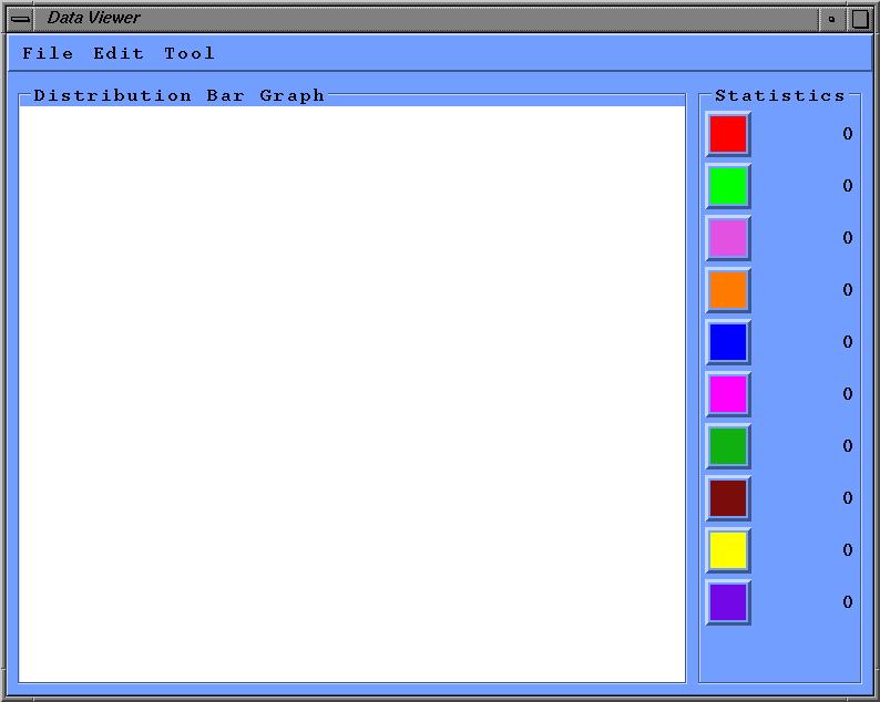
The main window, Data Viewer, of this application as shown in figure1, has a menu bar and two frames.
Figure 1. The appearance of the application’s main window.
There are three menu buttons, File, Edit, and Tool, on the menu bar; and under the menu bar, there are two frames, Distribution and Statistics. The larger frame on the left side of the main window is for displaying the histogram after filtering the input data file. The right frame with the title Statistics, which includes 10 color buttons and digits on the right side of each button. Those digits are the numbers of entries in the corresponding colored region of the histogram, and are set to be zero at the beginning.
The menu buttons on the menu bar are File, Edit and Tool. Under File menu, there is a submenu with four more buttons,
| Open: | When this option is selected, a dialog window, as in figure 2, will pop up and ask the user for the file name and the dimension of the data file. After the valid information is entered, the file is opened, the data are read in and screened, then finally a histogram will be shown to reflect the distribution of the data, and the number of entries of each colored area will be updated on the main window. |
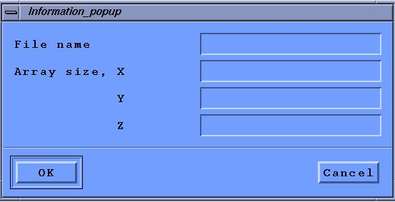
Figure 2. The appearance of the file information popup dialog box.
| Reset: | Redisplay the distribution histogram and reset the statistics shown in the main window to the information of the current active file. The previous selection is wiped out. |
| Close: | Close the current active file and the popup window for displaying images, clear the main window, and reset all flags and pointers. All the information about the previous selection and the active data file is cleared. |
| Exit: | When the button is selected, the program is exited. |
There is only one button under Edit menu,
| Select: | When the button is pushed, a dialog window is popped up, as shown in figure 3, and asks for the starting and ending range of the data interested. Then, the whole data set is screened again, and a new distribution histogram will be shown on the main window to reflect the result of the selection, and the statistics is updated. |
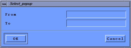
Figure 3. The appearance of the Select popup box.
Under Tool option, there is also one selection,
| Draw: | When the button is selected, a second window will pop up, as shown in figure 4; and the image of the current active data set will be plotted in that window. |
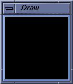
Figure 4. The appearance of the image rendering window.
Image Rendering
The images drawn in this application is done using OpenGL. The size of the popup window for rendering the image is twice the values of the x and y dimension of the input data file, if the x and y are less than or equal to100; otherwise, the window size is x by y. The image is rendered as points of size 2. And all the points are made somewhat transparent to show the points in the lower levels.
In the program, a utility function of Explorer on SGI workstation is used to generate the data of 256 colors for drawing points of different intensities. These colors are stored in a file and are read into a 256x3 array in the program. Each color is represented as the combination 3 floating-point numbers of red, green, and blue. To figure out which color to use in rendering a certain point, we take the intensity value of a point multiply by 255, then round it up to the next integer; then use that integer as an index to the array of colors. For example, a point with intensity of 0.0 use the first color in the array of colors, and a point with intensity of 1.0, take the last color.
Orthographic projection transformation is used to view the three-dimensional data set. OpenGL will take care of the conversion of three-dimensional model coordinates to screen coordinates, and other viewing problems, such as hidden face removal.
Error Handling
Before a file is opened for processing, pressing any button or making any selection will bring the following error message up, figure 5.
Figure 5. Error message for not specifying a data file.
Also, when the file information popup box is brought up, but no filename is entered, the same error message will appear again on the screen.
If the input filename, for example, test is not found, another error message will pop up, as in figure 6, with the incorrect filename concatenated in the message.
Figure 6. Error message for a file not found.
The error checking for the dimension of a file is loose; as long as the not all of them are zero, the program will accept. In that case, maybe only part of the data in the input file is read in and processed; or the incorrect array dimensions will cause distortion of the image. Otherwise an error message will pop up as in figure 7.
Figure 7. Error message of invalid file size.
For the error message popup boxes mentioned above, when OK is selected, the file information popup box, figure 2, will appear and ask the user to modify the existed file information. If Cancel is selected, the popup dialog box is closed and nothing is done.
If all the data in a selected data set are of the same value, a warning message, with the original intensity value, as shown in figure 8, will pop up to notify the user.
Figure 8. Warning message to notify the user of a homogeneous data set.
The selection of a data set is terminated when the difference of the starting and ending values is in the order of 10-6. Since float data type is used to store the normalized intensities, further dividing is meaningless, then a warning message will pop up, figure 9.
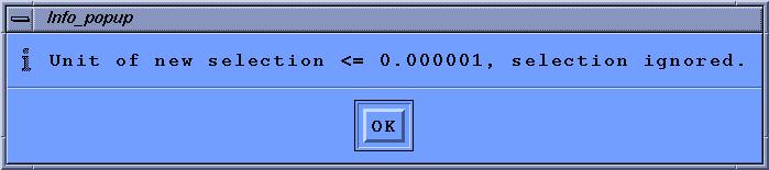
Figure 9. Warning message to notify the user that further selection is meaningless.
Other details
This project has to be complied on retriever or other workstations supports OpenGL GLU library. When compiling on those workstations in the graduate lab, an error message will tell you that it couldn’t find the library.
The ten colors selected to mark the ten segments of the distribution histogram are red, green, violet, orange, blue, magenta, limegreen, brown, yellow, and purple. The ten color buttons on the right side of the main window are related to the same colored region as in the histogram. User can click on any one of the color buttons to make a selection; it has the same result as clicking on Select under the Edit menu.
To normalize the whole input data or any selected data set, first we find the maximum and the minimum value of the data set, then for each data x in the data set,
Normalized x = (x – minimum) / (maximum – minimum).
When a certain range of data are selected, program will first filter the qualified data out from the input data set. Then, find the minimum and maximum of the selected data set, and follow the normalization process mentioned above to normalize the new set of data again, so when the selection is plotted, the new color corresponding to each point can show more detailed differences.
To count the number of entries of each interval, for example, 0.0 to 1.0 with increment of 0.1, and x is the intensity of an entry,
If 0.0 < x < 0.1, add one;
else if 0.1 < x < 0.2, add one;
else if 0.2 < x < 0.3, add one;
else if 0.3 < x < 0.4, add one;
else if 0.4 < x < 0.5, add one;
else if 0.5 < x < 0.6, add one;
else if 0.6 < x < 0.7, add one;
else if 0.7 < x < 0.8, add one;
else if 0.8 < x < 0.9, add one;
else if 0.9 < x < 1.0, add one.
To start the program, just type driver under the prompt, then hit return; a window, as in figure 1, will pop up. First, clip on the File button, select Open, then a window, as in figure 2, will be shown and ask for the input file information. Enter the proper information, for example as in figure 10, then click on OK. After reading in and screening the input file, the result will be shown in the main window, figure 11. To show the image of the data file, just push Tool button, and select Draw. The resulting image is shown in figure 12.
Figure 10. The file information popup box with valid file information.
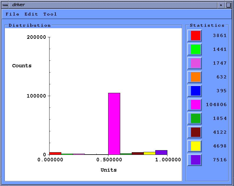
Figure 11. The result shown on the main window after a data file is been processed.
Figure 12. The image of the whole data file.
To select a subset of the data to be further examined either clip on one of the color buttons on the right side of the main window, to select a fixed range of data. Or click on Edit menu, press Select button, then enter the selection in the Select popup dialog. For example, the selected range is from 0.1 to 0.3, as in figure 13.
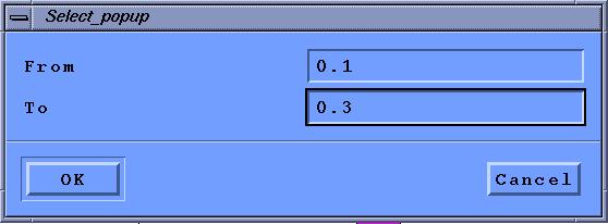
Figure 13. The select popup with inputs.
After the selection is entered, the popup window is closed, and a new bar graph will be shown in the main window to reflect the selection, figure 14.
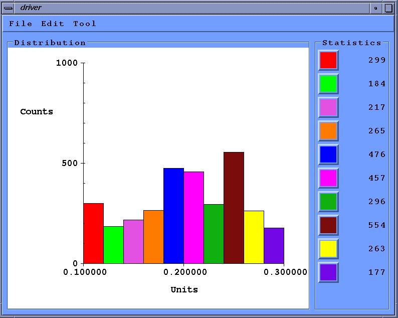
Figure 14. The result after a selection is made by press the first color button.
To show the image of the select data set, press the Draw button under the submenu of Tool, a popup window similar to the one in figure 7 will be displayed with the image of the current selected data in figure 15.
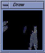
Figure 15. The resulting image of the selection.
User can make a more detail study of the data by making another selection of the current data shown in the main window; or press Reset button to bring the bar graph and statistics of the current active data file, and make new selection from there.
To open a new file, press Open button under File menu, this will bring the file information popup box in figure 10 back, and ask for new file information. Program will perform Close process before the file information popup box is brought up again. To end the application, just click the Exit button under the File menu.
Because of the different setup and the font supported on different workstations, the window, buttons, colors and the text will look slightly different on a different workstation.
Also, different data files have a different data format, the function get_input in file utility.c has to be modified to fit individual file format. Data viewer can also be used to filter any data file to find out the data frequency in that file, just remember to modify the get input utilities. And, plotting the data in this case won’t provide any further information.