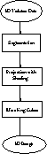
The SSD algorithm (sometimes called feature-extraction or
iso-surfacing) fits surface primitives such as polygons or patches to
constant-value contour surfaces in volume data [6]. This algorithm
consists of several principal steps [7]. The first step is
segmentation and the calculation of the normalized gradient vector at the
surface points. Segmentation is a procedure for partitioning the
three-dimensional(3D) gray-value data into foreground(objects) and background.
There are two ways to segment an image: edge detection (or surface detection)
and thresholding. If the 3D data form a rectangular space with unit cell of
dimensions a, b, and c, the gradient vector g=(g ,g
,g ,g
,g ) is estimated
from the density function by taking the central differences between the
densities, f(x
) is estimated
from the density function by taking the central differences between the
densities, f(x ,y
,y ,z
,z ), evaluated at the lattice points (x
 ,y
,y ,
z
,
z ).
).
¯
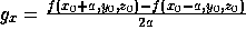

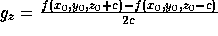
The gradient vector defined at each lattice point is trilinearly interpolated
over the voxel to give a local value of the gradient vector, g, at the desired
surface. To locate the surface, the density function is linearly interpolated
in the space (x,y,z) between the lattice points (x ,y
,y ,z
,z ) and
compared with the value C (threshold value) of the desired surface as the
surface of interest is f(x,y,z) = C.
) and
compared with the value C (threshold value) of the desired surface as the
surface of interest is f(x,y,z) = C.
The second step in the SSD algorithm is the shading procedure. Very realistic 3D-effects can be obtained by using Phong's shading formula.
¯

where I is the ambient light intensity, R
 is the
reflectivity light. I
is the
reflectivity light. I is the intensity of a point source of light, R
 is the diffuse reflectivity coefficient of the surface. R
 is the specular
reflectivity coefficient. The viewing distance is r, k is a constant, and the
angles
is the specular
reflectivity coefficient. The viewing distance is r, k is a constant, and the
angles  and
and  are explained by figure 3.
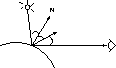
Figure 3: Angles in Phong's Formula
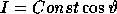
In this technique, only diffuse reflectivity is used. Therefore,
the last term of the above equation is set to zero. We assume no ambient
light, and that R is the same throughout the picture. The viewer is also
situated at infinity, which makes it possible to set the factor 1/(r+k) = 1.
With all these assumptions, Phong's shading formula is reduced to
is the same throughout the picture. The viewer is also
situated at infinity, which makes it possible to set the factor 1/(r+k) = 1.
With all these assumptions, Phong's shading formula is reduced to
¯
The third step is 3D surface reconstruction. In this step, the marching cubes algorithm is used to construct a surface. To summarize, the marching cubes algorithm includes the following steps: (1) Input the 3D data, the surface constant, view orientation, scale factors, cut planes, and nature of the cut surface. (2) Scan two consecutive slices and calculate an index formed by comparing the eight density values with the surface constant. (3) Tessellate each voxel configuration by retrieving edges from a precalculated table. (4) Interpolate the densities at the triangle vertices with respect to the desired surface density value. (5) Interpolate the voxel gradient vectors at the triangle vertices and normalize to find the vertex normal vectors. (6)Transform the vertices and the normal vectors to find the intensity at the triangle vertices. (7) Project triangles onto the view plane, and shade them by smoothly grading the intensity values.