CMSC 202 Lecture Notes: Asymptotic Analysis

A programmer usually has a choice of data structures and algorithms to use. Choosing the best one for a particular job involves, among other factors, two important measures:

• Time Complexity: how much time will the program take?
• Space Complexity: how much storage will the program need?

A programmer will sometimes seek a tradeoff between space and time complexity. For example, a programmer might choose a data structure that requires a lot of storage in order to reduce the computation time. There is an element of art in making such tradeoffs, but the programmer must make the choice from an informed point of view. The programmer must have some verifiable basis on which to make the selection of a data structure or algorithm. Complexity analysis provides such a basis.

Complexity

Complexity refers to the rate at which the storage or time grows as a function of the problem size. The absolute growth depends on the machine used to execute the program, the compiler used to construct the program, and many other factors. We would like to have a way of describing the inherent complexity of a program (or piece of a program), independent of machine/compiler considerations. This means that we must not try to describe the absolute time or storage needed. We must instead concentrate on a "proportionality" approach, expressing the complexity in terms of its relationship to some known function. This type of analysis is known as asymptotic analysis.

Asymptotic Analysis

Asymptotic analysis is based on the idea that as the problem size grows, the complexity can be described as a simple proportionality to some known function. This idea is incorporated in the "Big Oh" notation for asymptotic performance.

Definition: T(n) = O(f(n)) if and only if there are constants c₀ and n₀ such that T(n) <= c₀ f(n) for all n >= n₀.

Big Oh

If a function T(n) = O(f(n)), then eventually the value cf(n) will exceed the value of T(n) for some constant c. "Eventually" means "after n exceeds some value." Does this really mean anything useful? We might say (correctly) that n² + 2n = O(n²⁵), but we don't get a lot of information from that; n²⁵ is simply too big. When we use Big Oh analysis, we usually choose the function f(n) to be as small as possible and still satisfy the definition of Big Oh. Thus, it is more meaningful to say that n² + 2n = O(n²); this tells us something about the growth pattern of the function n² + 2n, namely that the n² term will dominate the growth as n increases. The following functions are often encountered in computer science Big Oh analysis:

• T(n) = O(1). This is called constant growth. T(n) does not grow at all as a function of n, it is a constant. It is pronounced "Big Oh of one." For example, array access has this characteristic. A[i] takes the same time independent of the size of the array A.

• T(n) = O(lg(n)). This is called logarithmic growth. T(n) grows proportional to the base 2 logarithm of n. Actually, the base doesn't matter, it's just traditional to use base-2 in computer science. It is pronounced "Big Oh of log n." For example, binary search has this characteristic.

• T(n) = O(n). This is called linear growth. T(n) grows linearly with n. It is pronounced "Big Oh of n." For example, looping over all the elements in a one-dimensional array would be an O(n) operation.

• T(n) = O(n log n). This is called "n log n" growth. T(n) grows proportional to n times the base 2 logarithm of n. It is pronounced "Big Oh of n log n." For example, Merge Sort has this characteristic. In fact, no sorting algorithm that uses comparison between elements can be faster than n log n.

• T(n) = O(n^k). This is called polynomial growth. T(n) grows proportional to the k-th power of n. We rarely consider algorithms that run in time O(n^k) where k is greater than 5, because such algorithms are very slow. For example, selection sort is an O(n²) algorithm. It is pronounced "Big Oh of n squared."

• T(n) = O(2ⁿ) This is called exponential growth. T(n) grows exponentially. It is pronounced "Big Oh of 2 to the n." Exponential growth is the most-feared growth pattern in computer science; algorithms that grow this way are basically useless for anything but very small problems.

The growth patterns above have been listed in order of increasing "size." That is,

O(1), O(lg(n)), O(n lg(n)), O(n²), O(n³), ... , O(2ⁿ).

Note that it is not true that if f(n) = O(g(n)) then g(n) = O(f(n)). The "=" sign does not mean equality in the usual algebraic sense --- that's why some people say "f(n) is in Big Oh of g(n)" and we never say "f(n) equals Big Oh of g(n)."

Example 1

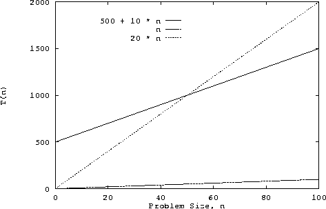
Suppose we have a program that takes some constant amount of time to set up, then grows linearly with the problem size n. The constant time might be used to prompt the user for a filename and open the file. Neither of these operations are dependent on the amount of data in the file. After these setup operations, we read the data from the file and do something with it (say print it). The amount of time required to read the file is certainly proportional to the amount of data in the file. We let n be the amount of data. This program has time complexity of O(n). To see this, let's assume that the setup time is really long, say 500 time units. Let's also assume that the time taken to read the data is 10n, 10 time units for each data point read. The following graph shows the function 500 + 10n plotted against n, the problem size. Also shown are the functions n and 20 n.

Note that the function n will never be larger than the function 500 + 10 n, no matter how large n gets. However, there are constants c₀ and n₀ such that 500 + 10n <= c₀ n when n >= n₀. One choice for these constants is c₀ = 20 and n₀ = 50. Therefore, 500 + 10n = O(n). There are, of course, other choices for c₀ and n₀. For example, any value of c₀ > 10 will work for n₀ = 50.

Example 2

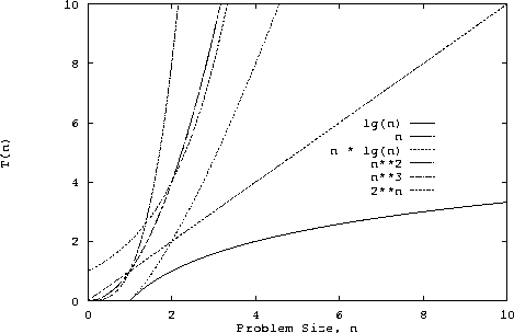
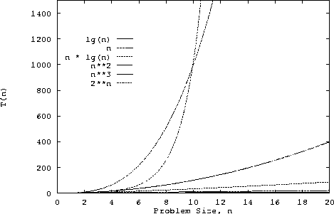
Here we look at the functions lg(n), n, n lg(n), n², n³ and 2ⁿ to get some idea of their relative "size." In the first graph, it looks like n² and n³ are larger than 2ⁿ. They are not! The second graph shows the same data on an expanded scale. Clearly 2ⁿ > n² when n > 4 and 2ⁿ > n³ when n > 10.

Example 3

The following table shows how long it would take to perform T(n) steps on a computer that does 1 billion steps/second. Note that a microsecond is a millionth of a second and a millisecond is a thousandth of a second.

Notice that when n >= 50, the computation time for T(n) = 2ⁿ has started to become too large to be practical. This is most certainly true when n >= 100. Even if we were to increase the speed of the machine a million-fold, 2ⁿ for n = 100 would be 40,000,000 years, a bit longer than you might want to wait for an answer.

Big Oh Does Not Tell the Whole Story

Suppose you have a choice of two approaches to writing a program. Both approaches have the same asymptotic performance (for example, both are O(n lg(n)). Why select one over the other, they're both the same, right? They may not be the same. There is this small matter of the constant of proportionality. Suppose algorithms A and B have the same asymptotic performance, T_A(n) = T_B(n) = O(g(n)). Now suppose that A does ten operations for each data item, but algorithm B only does three. It is reasonable to expect B to be faster than A even though both have the same asymptotic performance. The reason is that asymptotic analysis ignores constants of proportionality. As a specific example, let's say that algorithm A is

Algorithm A sets up faster than B, but does more operations on the data. The execution time of A and B will be

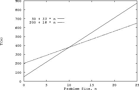
T_A(n) = 50 + 3*n + (10 + 5 + 15)*n = 50 + 33*n

T_B(n) =200 + 3*n + (10 + 5)*n = 200 + 18*n

Modified by Richard Chang, Fri Feb 13 14:25:48 EST 1998.